Tinker API Implementation on TPUs, 30B models and up to 20k context
Why I built a train-and-serve backend for the Tinker API on TPUs, and what it takes to run reinforcement learning on a 27-billion-parameter model at a 22,528-token context on a single v5p slice.
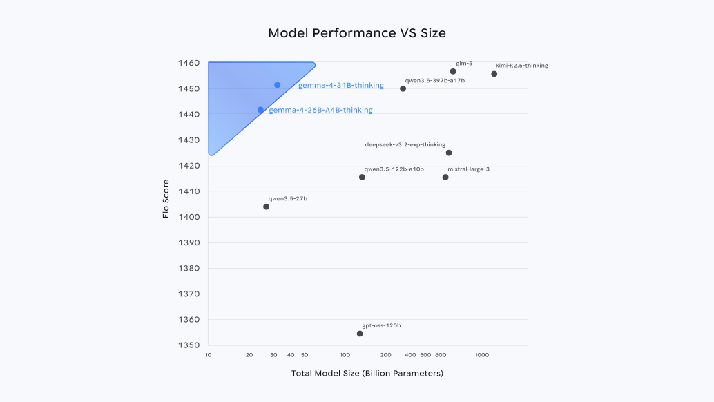
Really hard problems need a base model that already knows things: complex techniques, how to write good code, how to reason correctly. A 4B or 8B model does not clear that bar, and RL cannot supply what is missing — it can only reward attempts the model was already capable of making. So the starting point has to be around 30B.
Training a model that size used to mean full fine-tuning and the memory that comes with it. LoRA avoids that, and for RL it costs little: the update signal is sparse, because a whole rollout reduces to one score. Thinking Machines' analysis found LoRA matching full fine-tuning on policy-gradient RL even at very low rank.
Then there is the hardware. GPUs at this scale are hard to get. TPUs are easier, and the interconnect suits the job: chips are wired into a torus, so allocating a few dozen at once is normal, and the bandwidth between them is high enough to split a model across a host.
For the software I wanted the Tinker API. It is a small set of verbs, the algorithm stays in ordinary Python, and nothing in it refers to devices or meshes. But the hosted service is billed by usage, and most research runs get thrown away — sweeps, ablations, repeated attempts at a prompt format. That gets expensive.
In order to progress my research, I began working on this fork of SkyRL, which enables 30B model training at up to 20k context. The client code is unchanged; underneath it a MaxText model shards across one v5p host and vLLM serves from the others. Most of the difficulty was memory, which is the last third of this post.
Most of that work was memory, though not all of it. The pieces that mattered:
- Fused linear cross-entropy, with a hand-written gradient. At 20k tokens the
logits alone are 81.4 GB per chip, so the loss is computed in vocabulary tiles that are built,
read, and discarded — peak 2.0 GB, constant in context length. Tiling the forward pass is not
enough: ordinary reverse-mode autodiff saves each tile's output to reuse in the backward pass and
quietly reassembles the whole tensor. The fix is a
jax.custom_vjp, which replaces the reverse-mode rule JAX would derive with one that keeps only the hidden states and recomputes each tile on the way back. - One compiled shape for the entire run. XLA compiles a separate program per tensor shape and reserves a block of memory for each. Bucketing sequences to waste less padding cut padding from 60% to 22% and killed the run anyway, because six shapes meant six blocks.
- A leak inside MaxText. It records intermediate activations that outlive each compiled call — about 168 MB per tile, accumulating until no long run survived. Found by instrumentation, not by reading code.
- Qwen3.5 as a dense model in MaxText, which did not exist. A fork: dense-MLP decoder branch, model config, checkpoint converter, and two numerical bugs a normal-looking run would have hidden — the final norm needs Qwen3.5's zero-centered form, and mRoPE has to be off for text-only input.
- Adapter updates on a running vLLM. In RL the policy changes every step, so
the sampler has to pick up new weights constantly and restarting a server each time would
dominate the budget. TPU vLLM had no runtime-LoRA path, so that meant a fork of
tpu-inferenceadding the forwarders that let a versioned adapter be loaded and the previous one dropped in place, with the base weights and KV cache left warm.
The MaxText and tpu-inference changes are both general rather than specific to
this project, and I plan to upstream them.
It should be useful to anyone training a model around 30B at a context around 20k on text-only problems: code generation, reasoning, research-style search.
1. The machine
TPU Pod slices are available by number of TensorCores, which is neither the number of chips nor the number of physical machines.
| Slice | Chips | Hosts | Chips / host | HBM / chip | Total HBM |
|---|---|---|---|---|---|
| v5p-8 | 4 | 1 | 4 | 95 GiB | 380 GiB |
| v5p-16 | 8 | 2 | 4 | 95 GiB | 760 GiB |
| v5p-32 | 16 | 4 | 4 | 95 GiB | 1,520 GiB |
A host always has four chips, so a larger slice means more machines rather than denser ones. Each chip carries 95 GiB of high-bandwidth memory (HBM), which is roughly an H100's memory and still, as Section 10 shows, insufficient at long context. And each chip's two TensorCores appear to software as a single device: a v5p-16 ("16 cores") is 8 chips across 2 hosts, and JAX reports 4 devices per host.
2. Why I needed a new backend
SkyRL ships a JAX training backend that implements the model forward pass, the optimizer, and the sampling loop directly. It is readable and self-contained, and it was the right starting point. But it is a reimplementation, and on TPUs a reimplementation competes with a great deal of work that Google has already done and tuned:
- MaxText — reference LLM implementations written for TPUs, with the sharding annotations, attention kernels, and rematerialization policies already chosen and benchmarked.
- tunix — a post-training library that wraps those models with
LoRA (via
qwix), mesh construction, and checkpoint resharding. - tokamax — a kernel library underneath, supplying the fused attention primitives (MaxText can route its splash-attention scheduler through it).
The kernels I would have had to write
The concrete thing MaxText supplies is TPU kernels. Attention on a TPU is not a matrix multiply you write in JAX and hope the compiler handles; the fast implementations are hand-written in Pallas, JAX's low-level kernel language, and they are what separates a working model from a fast one.
| Kernel | Path | What it does | Status |
|---|---|---|---|
| Splash attention | training | Block-sparse flash attention for TPU: never forms the T×T attention matrix, so memory grows linearly in sequence length instead of quadratically. Indispensable at 20k tokens. | active |
| Ragged paged attention | sampling | Serves a batch of different-length sequences out of a paged KV cache without padding them to a common length — what makes continuous batching work. | active |
| Ragged attention | training | The same idea on the trainer: skip padded regions of a batch rather than computing and masking them. | available, off |
| tokamax splash scheduler | training | An alternative scheduler for the splash kernel, from Google's tokamax kernel library. | available, off |
Attention runs through a hand-written Pallas kernel on both halves of the stack, and neither is code I wrote: splash attention on the trainer through MaxText, ragged paged attention on the samplers through vLLM's TPU backend — where it is not a flag but the attention path itself. That pair is most of the reason this stack is built on MaxText and vLLM rather than on anything I would have had to write.
The two inactive rows are training-side, and the ragged one is not a flag away. The backend
does build a padding-aware mask, but the MaxText path discards it — MaxText applies causal
masking internally, and segment_ids is accepted by the adapter and never forwarded.
The kernel therefore sees a causal mask over the full length and has no way to know which
positions are filler; padded positions are dropped from the loss afterwards, once the compute has
already happened. Section 10 explains what it would take to reclaim that.
Sampling kernel: tpu_inference/kernels/ragged_paged_attention/v3/,
dispatched from layers/common/attention_interface.py.
The device mesh
The other thing I inherited is tunix's way of describing where a tensor lives. A
device mesh is a named grid of chips: instead of writing "shard this matrix
across four devices," you declare axes — fsdp, tensor,
data — give the mesh a shape over the physical chips, and annotate each tensor
with which of its dimensions map to which axis. The compiler derives every collective from
those annotations.
weights → sharded on fsdp // 13.5 GB per chip
batch → sharded on fsdp // one sequence per chip
This is why Section 3's choice is a one-line change rather than a rewrite, and why the "rows must be a multiple of the chip count" rule exists at all: the batch dimension is mapped to a mesh axis of size four, so it has to divide by four. tunix also carries the idea further than I use it — a mesh per role, so a trainer and a sampler can occupy different chips with weights resharded between them, which is the principled version of the trainer/sampler split I built by hand.
Writing my own forward pass would mean re-earning all of that by hand, per model
family. So I kept SkyRL's interface — the Tinker API server, which speaks
forward_backward, optim_step, and sample — and
replaced the engine underneath it with one that drives MaxText models through tunix.
The RL client never knows the difference.
Code: skyrl/backends/tunix_backend.py (~2,500 lines), plugged in via --backend tunix.
3. How the model is split across chips
Three ways to spread a model over four chips, and the vocabulary matters because the choice determines the shape of every tensor downstream.
| Strategy | Weights | Batch | Cost |
|---|---|---|---|
| DDP — distributed data parallel | full copy on every chip | split across chips | wastes memory; each chip stores all 54 GB |
| FSDP — fully sharded data parallel | split across chips, gathered per layer | split across chips | a gather per layer; cheap inside a host |
| TP — tensor parallel | every matrix split; chips cooperate on one sequence | not split | a collective inside every layer |
I use FSDP, and no tensor parallelism. Sharding the weights keeps 40 GB per chip free for activations. Skipping TP avoids a communication step inside every layer, and TP earns its keep only when a model cannot fit otherwise — a 27B model at bf16 (54 GB) fits in 95 GiB with room to spare.
= 2 × 27e9 / 4 = 13.5 GB // measured: 13.5 GB on every chip
4. The Tunix backend
Why not write against Tunix directly?
Tunix is a library: the natural way to use it is to import it and build a trainer inside its abstractions, in JAX. I wanted an API boundary in between instead, for three reasons.
LoRA is enough for this. An RL update carries very little information. Supervised learning supplies information on the order of the number of tokens in an episode; a policy gradient supplies O(1) — an entire rollout collapsing to a single advantage number. Thinking Machines' analysis makes that argument and finds LoRA matching full fine-tuning on policy-gradient RL at ranks as low as 1, on two conditions: that the adapter is not capacity-constrained, and that it covers the MLP layers rather than attention alone. Every run here trains a rank-32 adapter over attention and MLP and never touches the base weights — far above what the signal can carry, and what makes a 27B model trainable on a single host at all.
The internals stay switchable. When the algorithm talks to an API rather than to a trainer, what sits underneath becomes configuration. I can develop and debug against my own TPU server and run the same code against the hosted Tinker service when a run needs to be larger than my slice — a different base URL, not a different program. Section 9 is that property used as a test.
Many adapters over one base. The direction I want to explore next is multi-agent, and LoRA makes that cheap in the right way: a server holds many adapters against a single set of base weights (eight by default here), so several policies can be served and trained at once without several copies of a 27B model. Multiple bases would not fit; multiple adapters already do. That is an extension of the interface rather than a rewrite of it.
All of it was reachable because SkyRL had already reimplemented the Tinker API — the HTTP server, the futures, the request batching and barrier scheduling, the weight-sync semantics. That is a narrow contract:
| Verb | What it does |
|---|---|
forward_backward(datums, loss_fn) | accumulate gradients |
optim_step(adam_params) | apply them |
sample(prompt, n, params) | generate |
save_weights_and_get_sampling_client() | publish the policy to the samplers |
save_weights / load_weights | checkpoint and resume |
Writing a backend beneath that contract, rather than a trainer beside Tunix, meant inheriting all of the above and staying compatible with every client already written against it. Tunix is still here — qwix LoRA, mesh construction, the MaxText plumbing all sit inside the backend. It moved from being the framework to being a dependency behind an interface.
What the contract buys is visible in how little an algorithm has to say. This is a complete GRPO step:
sampling_client = await training_client.save_weights_and_get_sampling_client_async()

results = await asyncio.gather(*[
    sampling_client.sample_async(prompt=p, num_samples=group_size, sampling_params=sp)
    for p in prompts
])

datums = []
for result, prompt in zip(results, prompts):
    rewards    = [grade(seq) for seq in result.sequences]
    baseline   = sum(rewards) / len(rewards)
    advantages = [r - baseline for r in rewards]      # <- GRPO, in full
    if all(a == 0.0 for a in advantages):
        continue                                      # no signal in this group
    for seq, adv in zip(result.sequences, advantages):
        datums.append(tinker.Datum(
            model_input   = prompt.append(EncodedTextChunk(tokens=seq.tokens[:-1])),
            loss_fn_inputs = {"target_tokens": ..., "logprobs": seq.logprobs,
                              "advantages": ...},
        ))

await training_client.forward_backward_async(datums, loss_fn="importance_sampling")
await training_client.optim_step_async(adam_params)
Two lines are the algorithm. Nothing mentions a device, a mesh, a shard, or a compiler:
advantages is a list of Python floats, and switching to PPO is
loss_fn="ppo". Everything this post is about — sharding, packing, tiled
cross-entropy, compiled shapes — happens on the far side of
forward_backward, where the client cannot see it and does not have to.
That separation is what made the check in Section 9 possible at all: an unmodified published recipe, pointed at a different URL.
What the backend has to do
The backend's job is to make MaxText models honor those verbs. A few decisions shaped it:
- Load MaxText directly through
pyconfig, bypassing tunix's model-name registry, so any forked or unreleased model config can be loaded by path. Converted checkpoints are cached (Section 6). - Respect TPU shape rules. Sequence lengths round up to the 512-token attention block; batches pad to a multiple of the chip count. Both are handled inside the backend so the client can send whatever it has.
- Train adapters, not the model. LoRA (rank 32) via
qwix, targeting attention and MLP projections. Only adapter gradients exist, which is what makes a 27B model trainable on one host at all.
5. Sampling: vLLM, and inflight LoRA
An RL step spends most of its wall clock generating tokens, and generation is a different discipline from training — continuous batching, paged attention, careful KV-cache management. Rather than write that, I run vLLM on the sampling hosts.
The subtlety is that in RL the policy changes every step, so the sampler must be
updated constantly. Restarting a server per step would dominate the budget. Instead
each save_weights_for_sampler exports a standard LoRA adapter directory
and hot-swaps it into the running vLLM under a versioned name — load the new adapter,
unload the previous, keep the base weights and KV cache warm. The sampler tracks the
trainer within one step, and that is measurable: the divergence between the
policy that generated a token and the policy being trained stayed between
1×10⁻⁴ and 5.3×10⁻⁴ across a 180-step run.
How the sampler splits the model
The trainer uses FSDP. The sampler does not: vLLM runs tensor parallel across the four chips of its host, and the launcher derives that from the topology rather than being told:
more than one sampler host → independent replicas, a full model each // v5p-16: one replica · v5p-32: three
The trainer and the sampler make opposite choices on identical hardware, and for the sampler the reason is the KV cache. Tensor parallelism splits the weights, and what that buys is room:
KV cache = the ~88 GB per chip left over, pooled across the four
A full replica on a single chip would spend 54 of its 102 GB on weights before one sequence arrived. Splitting them four ways leaves nearly the whole host for cached attention state, which is the constraint that actually binds when a step is dozens of concurrent 20k-token rollouts. Decode is bandwidth-bound rather than arithmetic-bound, so the same split also means each chip reads a quarter of the weights per token; the activations exchanged per layer are one token wide.
That is the shape of the sampler numbers in Section 7: about 97 GB of HBM reserved against 1.7% of the TensorCores busy — memory reserved and bytes moved, not arithmetic performed.
Adapter path: tpu/vllm_tpu_server.py and a fork of tpu-inference
pinned at skyrl/v0.23.0-lora, so the runtime-LoRA hooks are source-installed rather
than patched at deploy time.
6. Caching, because the machine will be taken away
I run on preemptible (spot) slices: cheap, and reclaimed without warning. In practice mine lasted between one hour and two days. Any run longer than that has to survive losing its machine, which turns each expensive artifact into the same question: if this slice disappears, what should not have to be computed again?
| Cached artifact | Cost if lost | Where it lives |
|---|---|---|
| HuggingFace weights (54 GB) | ~35 min download | GCS mirror → local SSD |
| MaxText/orbax converted checkpoint | ~20 min conversion | GCS, keyed by model |
| vLLM XLA compilation cache | ~60 min cold compile | GCS, keyed by shape config |
| LoRA adapter + optimizer state | all training progress | GCS, every N steps |
| Graded rollouts for the current step | ~40–70 min of sampling | local, mirrored to GCS |
The last row is the one people forget. An RL step is sample, then train, and sampling is the long half. Preemption during the training half would otherwise throw away an hour of finished generation. Caching the graded rollouts mid-step means a replacement machine reloads them and goes straight to the gradient. With all five caches warm, a fresh slice goes from nothing to training in about 25 minutes, and the run resumes at the step it lost rather than the step it last checkpointed.
7. The training loop: synchronous, then pipelined
The first working version was the obvious one. Sample the whole batch, wait, train on it, wait, repeat. It worked, and it wasted half the machine: while the sampling hosts generate, the training host idles, and vice versa.
The pipelined version streams finished minibatches to the trainer as they are graded. Training begins as soon as the first wave lands, and the sampling of later waves hides inside the gradient math of earlier ones. Measured on a v5p-16 with Qwen3-8B, 1024 rollouts per step:
| Configuration | s / step | Speedup |
|---|---|---|
| Synchronous loop, micro-batch 8 | 330 | — |
| Micro-batch 32, adapters published directly (no archive round-trip) | 290 | 1.14× |
| Pipelined: streamed minibatches, concurrent sampling | 210 | 1.57× |
Inside a 210-second step: gradient waves take ~130 s and pace everything (sampling's ~95 s hides entirely inside that window), adapter export and load take ~45 s of pure I/O, and the optimizer step itself takes 0.1 s. The proportions are what matter: the gradient update is essentially free, and nearly all of a step is spent moving data and waiting on generation.
Utilization: nothing here is compute-bound
A sidecar samples each chip's counters during training and logs them alongside the run. The numbers say where the remaining performance is.
Two different bottlenecks. Decode is memory-bound by nature — generating one token reads the whole model and does almost no arithmetic with it — so 1.7% TensorCore is close to expected, and vLLM's job is to keep enough sequences in flight to hide it. The trainer's 15–21% is the more interesting figure: it is not FLOP-limited but pipeline-limited, waiting on requests, results, and adapter I/O. That is what the pipelined loop attacks, and why the next unclaimed gains are also structural — one-step-off-policy sampling, and an in-place adapter reload to cut the 45-second sync.
Parameters that actually matter
| Knob | What it trades |
|---|---|
GROUP_SIZE × GROUPS_PER_BATCH | rollouts per step: gradient quality vs. step time (I use 8×32 and 16×32) |
STREAM_NUM_MINIBATCHES | how finely sampling is streamed to the trainer; more overlap vs. more per-call overhead |
TRAIN_MICRO_BATCH_SIZE | sequences per gradient call; the single biggest memory lever |
LORA_RANK | adapter capacity (32 throughout) — also sets gradient and optimizer size |
MAX_TOKENS / context window | the subject of Section 10 |
8. Making Qwen3.5 exist in MaxText
I wanted two strong open models: Gemma-4-31B and Qwen3.5-27B. Gemma was straightforward — MaxText already ships a reference implementation, so it was a matter of adapter plumbing. Qwen3.5 was not implemented at all, and its architecture is unusual enough to be interesting: a hybrid stack where three of every four layers use linear attention (a gated DeltaNet) and every fourth uses full attention, with a 248,320-token vocabulary.
I added it in a MaxText fork: the dense-MLP branch in the decoder, a model config, and a HuggingFace→orbax converter mapping. Most of the effort then went to a subtler problem — proving the port was numerically correct. If the trainer's model disagrees with the sampler's, RL still runs; it just quietly optimizes the wrong objective.
A three-way log-probability comparison (the MaxText port, the HuggingFace reference, and the vLLM sampler), together with a per-layer bisection, found three bugs. They failed in different ways, which is why all three are listed here.
| # | Bug | Why it was needed |
|---|---|---|
| 1 | Final norm used plain RMSNorm; Qwen3.5 uses the zero-centered form (1+w)·x̂ |
The expensive one. A flat ~2 nats/token divergence that per-layer comparison cannot see — the reference exposes hidden states before the final norm, so every layer matches and only the output is wrong. |
| 2 | Multimodal RoPE must be disabled for text-only inputs | MaxText's mRoPE rotates the full head dimension, ignoring the partial-rotary factor this model expects. Silently wrong positions, not a crash. |
| 3 | The LoRA tracing batch must divide the FSDP mesh | The gated-DeltaNet layers shard their batch internally; a trace batch that does not divide evenly fails at adapter-injection time. A shape rule, not a math bug. |
The payoff is measurable: at step 0 the sampler and trainer disagreed by 1.7×10⁻⁴ nats — the cleanest parity of any model I brought up, and the evidence that the port was right before a single gradient was taken.
9. Does it learn?
I validated on mathematical reasoning with verifiable rewards: the model answers competition-style problems, correct answers are rewarded, and accuracy is tracked on a held-out set.
First Qwen3-8B from a cold start, 180 steps on a v5p-16 — held-out accuracy went 1.2% → 77.4%. That run also survived a preemption at step 60 and resumed on a fresh machine with optimizer state intact, which was the real test of Section 6.
Then two 30B-class models on the same recipe and the same hardware — Qwen3.5-27B and gemma4-31B, each 256 rollouts per step, rank-32 LoRA, 2e-5, 512 tokens, 180 steps:
| Held-out accuracy | step 0 | 20 | 40 | 60 | 80 | 100 | 120 | 140 | 160 | 179 |
|---|---|---|---|---|---|---|---|---|---|---|
| Qwen3.5-27B | 37.2% | 73.4% | 84.8% | 85.6% | 86.4% | 83.2% | 86.0% | 87.0% | 86.2% | 86.4% |
| gemma4-31B | 62.4% | 65.6% | 68.6% | 71.8% | 72.8% | 77.0% | 77.2% | 78.4% | 81.0% | 80.4% |
gemma4-31B is also the best evidence for Section 6. That run survived four spot preemptions — each time the supervisor recreated the machine and resumed from the last checkpoint in GCS, with the step count continuous across all of them — for 7.1 hours of training wall clock at a mean of 142 s per step.
Two things are worth recording against it. Its adapters ship through vLLM's native LoRA path
under composite names (model.language_model.layers.N), and MaxText's six-layer
grouped scan de-interleaves as hf_layer = stack_idx × 6 + k; because the global
layers carry no v_proj, a correct adapter is 820 tensors rather than 840. Get the
names or the mapping wrong and it loads successfully and does nothing. And its sampler-trainer
KL drifted from 0.026 early to about 1.0 by the end (mean 0.39) without denting the eval curve —
benign over 180 steps, but the Qwen run held inside [1×10⁻⁴, 5.3×10⁻⁴],
and that is the behaviour I would want on anything longer.
Against a published reference
The client in all of this is not my code. It is the
Tinker Cookbook
math-RL recipe run unmodified — the same module, the same defaults — with two
arguments changed: model_name, and a base_url pointing at my server
instead of the hosted API. The training code never learns it is talking to my TPUs.
Thinking Machines publishes a result for that recipe, which gives an outside number to check against:
python -m tinker_cookbook.recipes.math_rl.train env=math \
  model_name="Qwen/Qwen3.5-9B" group_size=16 groups_per_batch=64 \
  learning_rate=2e-5 max_tokens=512

# after 180 steps: "test/env/all/correct": 0.838| Run | Model | rollouts/step | steps | held-out |
|---|---|---|---|---|
| Cookbook (hosted Tinker) | Qwen3.5-9B | 16 × 64 = 1024 | 180 | 83.8% |
| this stack, v5p-16 | Qwen3-8B | 16 × 64 = 1024 | 180 | 77.4% |
| this stack, v5p-16 | Qwen3.5-27B | 8 × 32 = 256 | 180 | 86.4% (peak 87.0%) |
| this stack, v5p-16 | gemma4-31B | 8 × 32 = 256 | 180 | 80.4% (peak 81.0%) |
Learning rate (2e-5), token budget (512), LoRA rank (32), loss function and step count are identical across all four rows. The rest is not controlled, and I would not read it as a head-to-head: the Qwen3-8B row is a different model generation, and the two 30B rows train on a quarter of the batch — two differences that push in opposite directions. What the table does establish is that the same recipe pointed at my backend lands in the same band as the published number rather than somewhere anomalous.
10. The 22,528-token wall
Everything above happens at a 512-token generation budget. That is enough for math answers and nowhere near enough for the actual target: a model that reasons at length — thinking for thousands of tokens before writing a program that gets executed and scored.
Raising the context from 512 to 22,528 tokens broke the system in five distinct ways. This is the part worth reading, because the failures were not "out of memory, use less" — they were structural, and each fix is a small piece of engineering with a clean idea in it.
Where the memory actually goes
Start with the arithmetic. A training step must, for every token, compare the model's predicted distribution against the token that was actually sampled. The naive way materializes the full distribution:
at 512 tokens: 4 × 512 × 248,320 × 4 = 2.0 GB // comfortable
at 20,480: 4 × 20,480 × 248,320 × 4 = 81.4 GB // on a 95 GiB chip that already holds 13.5 GB of weights
Qwen3.5's vocabulary of 248,320 is what makes this severe. The logits tensor grows linearly in context length and is multiplied by a quarter of a million — at 20k tokens it alone exceeds what the chip has left, before counting the activations of 64 transformer layers or the copy that computing a log-softmax would produce.
1 · Score log-probabilities on the training chips
RL needs the log-probability of tokens that were already generated. The natural place to get them is the inference server — but vLLM's TPU backend crashes when asked to return them for long prompts. So I moved that computation onto the training host, where the model already lives, jitted it, and gathered only the target token's value inside the compiled program rather than returning a full distribution. The scoring path also has to pad its batch to the chip count, exactly like training.
2 · Pack micro-batches by token budget, not sequence count
"Eight sequences per batch" is meaningless when sequences range from 1,000 to 20,000 tokens. I pack by total tokens instead:
Memory then depends on a quantity I control, rather than on whatever lengths the model happened to produce.
3 · Never materialize a log-softmax
The standard way to get a token's log-probability is log_softmax(logits)[target],
which allocates a second tensor the size of the first. The identity
= x[i] − log Σ exp(x[j]) // log of a quotient
= x[i] − logsumexp(x)
saves the entire tensor. The two sides are equal by definition, but they cost different
amounts: the left-hand side produces a vector with one entry per vocabulary token —
248,320 numbers, of which exactly one is ever read — while the right-hand side is a gather
(x[i]) minus a scalar reduction. The vocabulary axis is summed away rather than
written out, and XLA fuses the reduction into the preceding operation, so the intermediate
never lands in memory at all.
The numerics are unchanged.
A stable logsumexp is computed as m + log Σ exp(x − m)
with m = max(x) — the identical shift that log_softmax applies
internally. Same arithmetic, same floating-point result, one fewer tensor. This one line is
what made a KL-regularized run fit at all.
4 · Fused linear cross-entropy: the logits never exist
The identity in (3) removes the copy, but the logits themselves are still built. The real fix is to never form them: split the tokens into tiles, and for each tile project hidden states to vocabulary, take the one number needed, and throw the tile away.
versus 81.4 GB for the whole batch — a 40× reduction, constant in T
This is where a subtlety cost me three attempts. Tiling the forward pass is easy; the problem is the backward pass. If you write the loop with a standard scan — even wrapped in gradient checkpointing — automatic differentiation saves every tile's logits so it can reuse them, stacks them back together, and reconstructs the exact 81 GB tensor you were avoiding. The loop looks tiled and is not.
The fix is a custom gradient: it tells the compiler that the forward pass keeps only the hidden states, and that the backward pass should recompute one tile's logits at a time. Peak memory is then one tile in both directions, enforced by the gradient definition itself rather than left to the compiler's discretion.
Code: _flce_target_logprobs in skyrl/backends/tunix_backend.py —
a jax.custom_vjp whose forward residual is deliberately the hidden tiles, never the logits.
5 · Keep the compiler to one shape
XLA compiles a separate program for every tensor shape it is given, and each program reserves its own block of memory to work in. Feed it many shapes and those blocks pile up — tens of gigabytes each — until a new shape has nowhere left to load. Measured on this workload, the reserved block grows at roughly
I tried the clever approach first — bucketing sequences into a ladder of lengths to waste less padding — and it backfired: padding dropped from 60% to 22%, but six live memory blocks replaced one, and the run failed the moment a seventh shape appeared. What worked was the simpler approach, and the one MaxText and tunix follow by convention: pad everything to a single shape. One program, one reserved block, for the whole run. Roughly 60% of the tokens in a tile are then padding — real compute, spent on nothing — and it is still the better trade, because the alternative does not run at all.
segment_ids.
Fixing that alone would not buy much, because attention is not where the waste sits. The q/k/v/o
projections, the MLP and the cross-entropy tiles are per-token dense operations with no mask to
consult, so a padded position costs exactly what a real one costs in every one of them. The
actual fix is sequence packing: concatenate several real sequences into one row
behind a block-diagonal mask, so the filler becomes other sequences' tokens and the dense layers
do useful work. That requires segment_ids plumbed through to MaxText's decoder,
which is deeper than a configuration change, and it is the largest unclaimed win left here.
6 · The leak that hid behind all of it
With one shape and fused cross-entropy, a training step still died — deterministically, around the 55th tile of 92, always with the same "cannot allocate" message. Memory grew ~170 MB per tile, with nothing in my code to explain it.
Instrumentation settled it. Logging every live array on the chip every ten tiles showed
watched one shape's count climb: [4, 16384, 5120], one more copy per tile,
forever. Those are hidden states — and MaxText's decoder sows them into the model
object as a debugging convenience. Under JAX's functional-object wrapper, changes a model
makes to itself during a compiled call persist after it. Ninety-two calls, ninety-two
retained copies. The fix is one line, executed after each tile:
nnx.pop(model, nnx.Intermediate) # discard sown intermediatesMemory went flat at 29.1 GB across all 92 tiles, and the first end-to-end training step completed. Two related fixes landed with it: gradient accumulation moved inside the compiled function with its buffer donated (the previous version kept three copies of the gradients alive), and the out-of-memory handler learned to retry gently before evicting the compiled program — the old handler turned a single transient failure into an unrecoverable spiral by discarding the very program it needed to reload.
11. Cookbook
Everything in this post runs from one repository. The recipes below create and tear down their own slices, so the only prerequisites are credentials and capacity.
Clone with submodules — the tpu-inference fork carries the runtime-LoRA
hooks from Section 5, and is source-installed rather than patched at deploy time:
git clone --recurse-submodules https://github.com/SachinKonan/SkyRLTpu.git
cd SkyRLTpu
Authenticate. TPU v5p capacity has to exist in the default project — a v5p-16 for the math-RL recipe, a v5p-32 for long context:
gcloud auth login
gcloud config set project <your-gcp-project>

export ZONE=<zone-with-v5p-capacity>
Then point the three caches of Section 6 at a bucket you own. Skipping this costs roughly an hour of cold compilation and download on every fresh slice:
export TUNIX_MAXTEXT_CKPT_CACHE_GCS=gs://<your-bucket>/skyrl-maxtext-ckpts
export HF_CACHE_GCS=gs://<your-bucket>/hf-cache
export VLLM_XLA_CACHE_GCS=gs://<your-bucket>/vllm-xla-cache
Commands are invoked through uv; the scripts provision the hosts themselves.
The 180-step run from Section 9. One command owns the whole lifecycle — queued-resource creation, colocated bring-up, client launch, and resume after preemption.
./tpu/autoresume_run.sh tpu/runs/qwen35-27b.envThe env file is the entire specification:
MODEL_NAME=Qwen/Qwen3.5-27B
TUNIX_MAXTEXT_MODEL_NAME=qwen3.5-27b
TUNIX_MAXTEXT_PIP_SPEC="maxtext @ git+https://github.com/SachinKonan/maxtext.git@skyrl/qwen35-dense"
TRAIN_WORKERS=0            # host 0 trains
VLLM_WORKERS=1             # host 1 samples
TRAIN_MICRO_BATCH_SIZE=8
GROUP_SIZE=8  GROUPS_PER_BATCH=32   # 256 rollouts / step
MAX_TOKENS=512  LORA_RANK=32  LEARNING_RATE=2e-5
STREAM_NUM_MINIBATCHES=8   # pipelined overlap
RENDERER_NAME=qwen3_5_disable_thinking
MAX_STEPS=180 SAVE_EVERY=20 EVAL_EVERY=20The configuration this post's second half exists to support: the model thinks for thousands of tokens, writes a program, and the program's measured quality is the reward. Server first — note the single fixed shape and the fused cross-entropy tile:
TINKER_BACKEND=tunix  MODEL_NAME=Qwen/Qwen3.5-27B \
TRAIN_WORKERS=0  VLLM_WORKERS=1,2,3 \
TUNIX_UNIFORM_SEQ_LEN=20480 \    # one program shape, ever  (fix 5)
TUNIX_TRAIN_TOKEN_BUDGET=81920 \ # 4 sequences x 20480      (fix 2)
TUNIX_FLCE_TILE_SIZE=2048 \      # fused linear CE tile     (fix 4)
TUNIX_MAXTEXT_KWARGS='{"num_vocab_tiling": 8}' \
  ./tpu/start_colocated_vllm_tinker.sh
Then the client, on the training host:
EXPERIMENT_NAME=erdos-qwen35  TTD_ENV=erdos_min_overlap \
PHASE1_MAX_TOKENS=15872  CONTEXT_WINDOW=20480  TTD_TRAIN_MAX_SEQ=20480 \
GROUP_SIZE=16  GROUPS_PER_BATCH=32  KL_PENALTY_COEF=0 \
  bash tpu/run_ttd_on_tpu_host.sh
PHASE1_MAX_TOKENS is the thinking budget; the remaining ~4.6k tokens are
reserved so the model can always finish writing its program. Sizing that tail is empirical —
I measured real program lengths (1.2k–5.3k tokens) and left room for the largest.
12. What next
Two directions are open, and they are hard for different reasons. One is a serving problem I partly solved and do not fully trust; the other is a capacity problem I have not attempted.
Mixture-of-experts, and where adapters attach
Everything above trains dense models. The obvious way to get more capability per unit of compute is a mixture-of-experts model, where each token is routed to a few of many expert networks. I built the path for gpt-oss-20b and it works, but it required breaking an assumption that holds everywhere else in this stack.
The assumption is that a LoRA adapter can be attached to a layer. In a dense model, vLLM wraps each target layer so the adapter is applied at runtime — which is what makes hot-swapping cheap, and is the mechanism Section 5 depends on. In an MoE model on TPU, vLLM fuses all experts into one large tensor and runs them as a single batched operation, because doing otherwise would be far slower. There is no per-expert layer left to wrap: the abstraction the adapter needs has been optimized away.
It is worth the trouble because adapting attention alone is not equivalent. The LoRA result in Section 4 holds only when the adapter covers the MLP layers — and in a mixture-of-experts model, the MLP is the experts. Skipping them is precisely the capacity-constrained case the analysis warns about, so an MoE model trained through attention only is not the same experiment.
The resolution is to split the exported adapter in two. The attention projections ship as a
standard PEFT directory and take vLLM's native path. The expert factors ship as a sidecar and are
merged into the fused tensor at load time, through a custom collective RPC —
apply_moe_lora_deltas — that hands each worker its factors and adds them in place.
Getting there also meant disabling vLLM's own MoE-LoRA wrapper on TPU, which fails to boot against
bf16 experts.
Code: tpu/vllm_tpu_server.py plus the tpu-inference fork
(merge extraction, donated in-place adds, equivalence tests against incremental merges).
The instability I have not solved
This path runs, and it is not yet trustworthy. Sampling occasionally returns NaN log-probabilities for individual tokens. Downstream that is catastrophic rather than merely noisy, because the RL loss exponentiates a difference of log-probabilities:
sampling_logprob = −1e4 // the clamp standing in for NaN
→ ratio = exp(1e4) = inf // one token poisons the batch
The current defense is three layers deep, and every layer is containment rather than a cure.
NaNs are clamped to a sentinel value at the source in the fork; any token carrying that sentinel
has its loss weight zeroed and its value neutralized (a zero weight is not enough — inf × 0
is NaN inside a compiled function); and non-finite optimizer updates are skipped outright. The
gradient is protected. What I still cannot say is why the fused MoE path produces NaN
log-probabilities in the first place — whether it is an overflow in the bf16 expert matmuls, the
router, or the merge itself. Until that is answered I would not run a long MoE job unattended.
Larger models: is tensor parallelism the answer?
Nothing here has been run on a model larger than 27B on my own hardware. (A 120B model appears in my results, but those runs used hosted infrastructure, not this stack.) The arithmetic for attempting it is simple enough to state:
C = 4 (1 host) → 60 GB/chip // ~35 GB left; a 20k memory block alone needs 37 GB — no
C = 8 (2 hosts) → 30 GB/chip // ~65 GB left — comfortable
C = 16 (4 hosts) → 15 GB/chip // ample
So tensor parallelism is probably not what I need. TP earns its place when a single tensor is too large for one chip; here no individual tensor is the problem, total capacity is — and capacity is what sharding across more chips buys. The natural move for 120B is multi-host FSDP over two or four hosts, not a different parallelism strategy within one.
That is also the honest description of the blocker: my backend trains on a single host by construction, and refuses more. Multi-host is not a missing flag but a missing mechanism — every process must execute the same compiled program in lockstep, which means a coordinator broadcasting each operation to workers. SkyRL's original JAX backend already implements exactly that pattern, so the work is porting it rather than inventing it.
I did try tensor parallelism, out of curiosity and because it would have shrunk the memory footprint of a training tile. Two configurations, two different failures: splitting four chips as 2×2 left 0.7 GB free after loading the model, against 27–29 GB under plain FSDP, for reasons I never isolated; and a 4-way tensor split failed inside the attention kernel, which requires its mask blocks to divide evenly across devices — the same divisibility rule from Section 3, reappearing one level down. Both are recorded as measurements rather than conclusions.
Built on SkyRL, MaxText, tunix, and vLLM. Measurements come from runs on v5p-16 and v5p-32 slices; the model-parallelism, memory, and timing figures quoted here were instrumented on those runs rather than estimated.